Where Can Pregnant Women Go?
metadata
- keywords:
- published:
- updated:
- Atom Feed
Recently I travelled to Colorado with a pregnant woman. The NHS guidance on exercise in pregnancy says:
Don’t exercise at heights over 2,500m above sea level until you have acclimatised: this is because you and your baby are at risk of altitude sickness.
 This led to some interesting discussions, particularly because a lot of Colorado is above 2,500m ASL due to the fact that the Rocky Mountains run straight through the state. One day, whilst visiting Rocky Mountain National Park we found a valley that was less than 2,500m ASL (specifically Moraine Park at 8,160ft ASL or 2,487m ASL) but the road to the valley briefly went over 2,500m ASL. In the end, we decided to still drive to the valley but it got me thinking: how common is it for there to be places that are less than 2,500m ASL but which you cannot access on land/water without going over 2,500m ASL to get there? Obviously you could cheat by flying there in a pressurised cabin - but that isn’t a fun programming project.
To solve this problem I wrote WCPWG (Where Can Pregnant Women Go?), which uses FORTRAN for the hardcore searching and Python for data conversion and pretty output. The basic method is:
- load elevation data provided by the GLOBE project
- set the top-left corner (the North Pole) as ‘accessible’
- loop over all pixels and set them as ‘accessible’ too if they are less than or equal to 2,500m ASL and if one of the (up to) eight surrounding pixels is also ‘accessible’
- continue looping over the world until no more pixels are marked as ‘accessible’
This method can be seen in action in the animation below. You can see that the first pass (which goes left-to-right scanning down each column one-by-one) finds most of the accessible places in the world and that subsequent passes just refine some very particular places (the north-western edge of the Tibetan Plateau is perhaps the most obvious).
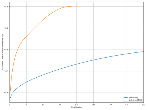
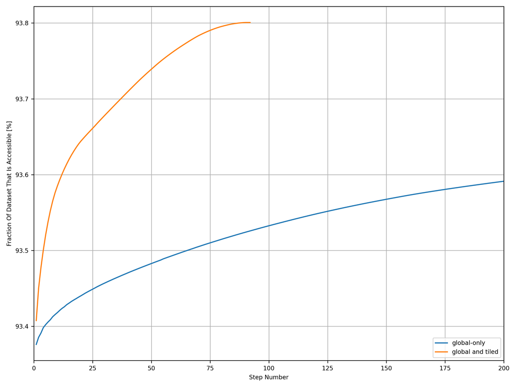
Pretty quickly it became apparent that it was going to take ages to find all of the accessible places. You can see that the first pass found the vast majority of the accessible places, but that some nooks and crannies were going to take an awfully long time to converge. It seemed silly to keep on scanning the whole world if only a few small places weren’t yet converged. I therefore wrote a second version that split the world up into small tiles and iterated each one separately. I still needed a global pass to ensure that accessible regions could cross across tile boundaries, but it certainly seemed to help. The convergence of the two different strategies can be downloaded: the CSV file for global-only and the CSV file for global and tiled.
I then wrote a simple Python script to plot the CSV files (shown below).
1 2 3 4 5 6 7 8 9 10 11 12 13 14 15 16 17 18 19 20 21 22 23 24 25 26 27 28 29 30 31 32 33 34 35 36 37 38 39 40 41 42 43 44 45 46 47 48 49 50 51 52 53 54 55 56 57 58 59 60 61 62 63 64 65 66 67 68 69 70 71 72 73 74 75 76 77 78 79 80 81 82 83 84 85 86 |
|
checkout the “main” branch).As you can see in the plot below it was going to take ages to find them all if I did not split the world up into tiles every step.
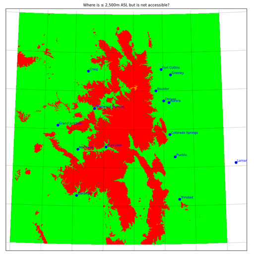
The FORTRAN program created a nice map of the mountains in Colorado (shown below). You can see all of the places that are forbidden in red and accessible in green. If you look very carefully on the eastern edge of the Rockies (just to the west of Denver and Boulder) there are one or two orange pixels - these are places which are less than 2,500m ASL but which cannot be accessed by land/water without going over 2,500m ASL. There is a particularly large orange region on the west of the Rockies (north-east of Glenwood Springs).
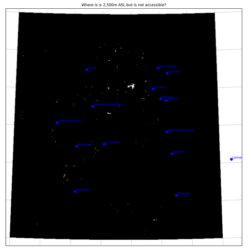
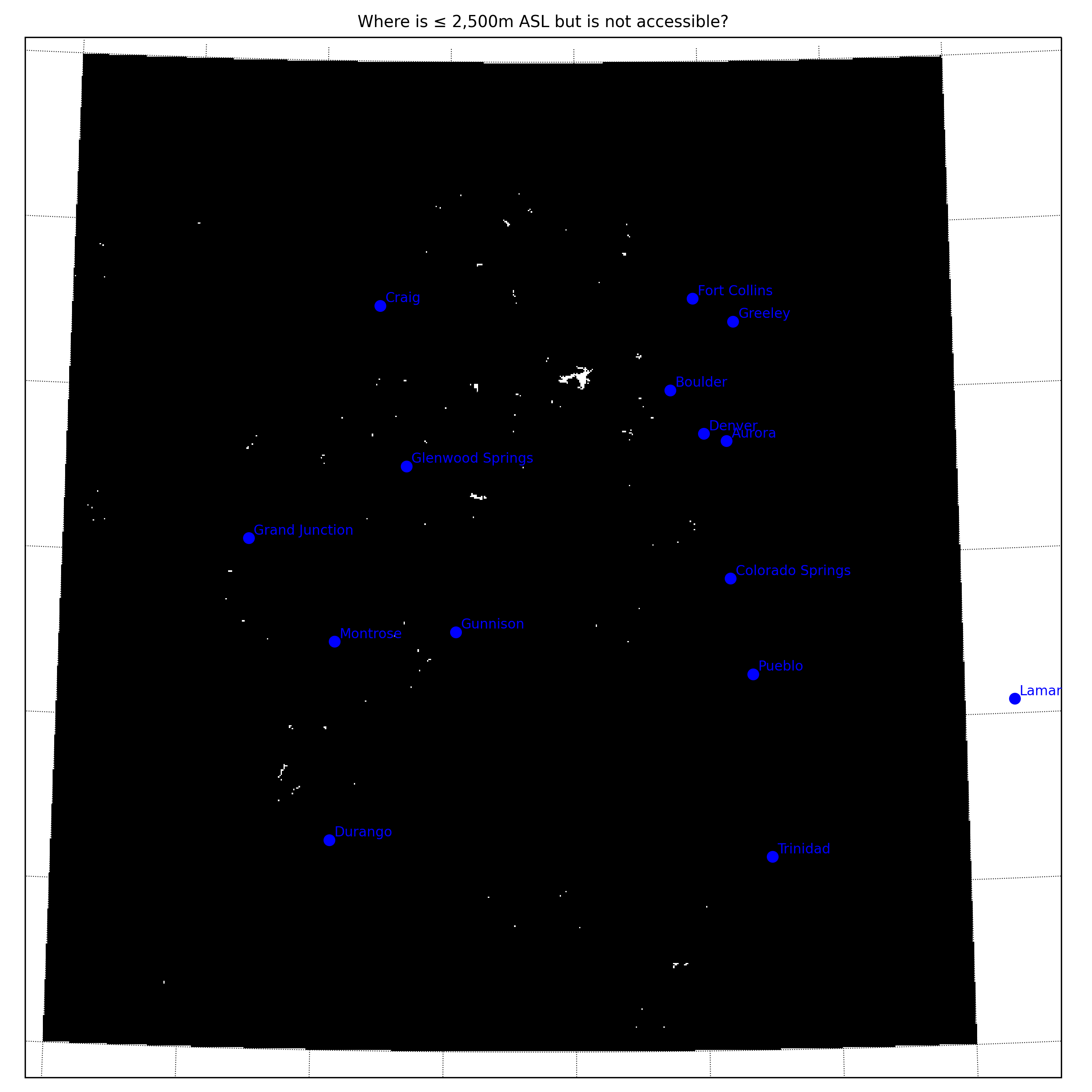
These orange regions are perhaps more easily observed in the black-and-white plot below.
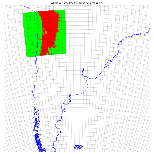
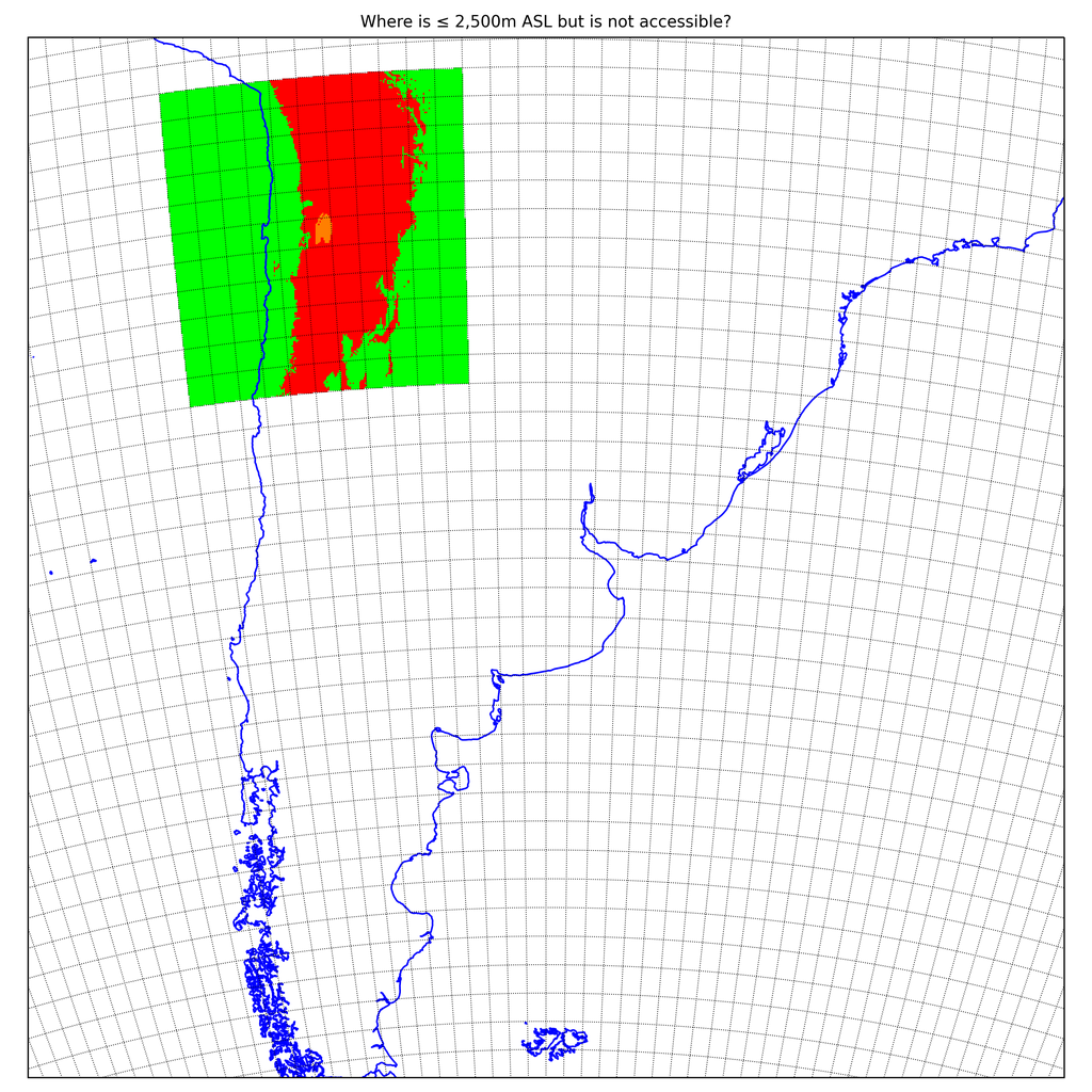
Finally, when I looked at the whole world as a 43,200 px × 21,600 px (933.1 Mpx) image (which is included at the very bottom of this blog post) one region jumped out in particular: Salar de Atacama. This is a large salt flat in the Atacama Desert and it is the largest salt flat in Chile. The average elevation is about 2,300m ASL which means that the surrounding mountains don’t have to be that much taller for it to be blocked off and marked as inaccessible. You can see this clearly in the plot below.
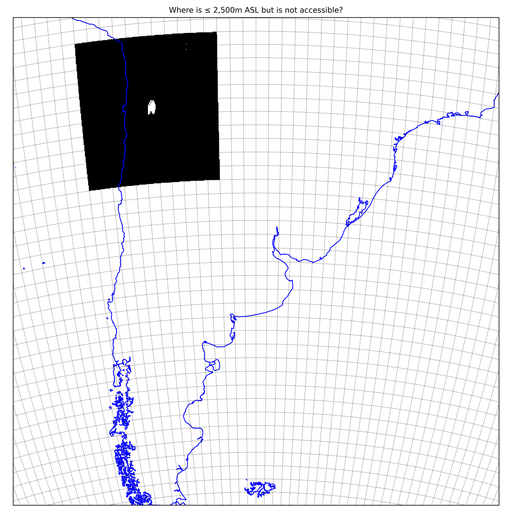
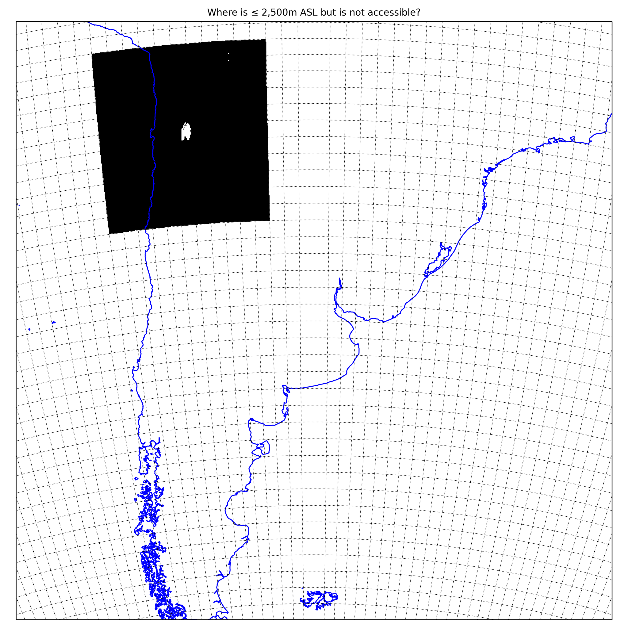
Or perhaps even more easily in the black-and-white plot below.
In conclusion, there are a few places in the world that are less than 2,500m ASL but which are not accessible without going over 2,500m ASL if you are travelling by land/water. Most of these are tiny, with the odd exception of a valley or two in a high mountain range such as those found in Colorado. The largest contiguous region by far that is inaccessible is the Salar de Atacama in Chile with an area of around 3,000km2. For completeness I have included the two different types of maps for the entire globe below:


As a curious aside: this exact same algorithm could be used to answer the question of “which valleys wouldn’t be filled in by water if the sea level rose by 2,500 metres”; stay tuned …