Reliably Buffering A Shape By A Geodetic Distance
This post has been a long time coming and it is broken down into sections:
I have also included some discussion on the background principles associated with this topic, such as great circles and Tissot’s indicatrix.
§1 Introduction
On the 25th of February 2017 I committed my first implementation of Vincenty’s formulae into my Python 2 module. Three and a half years later, on the 21st of August 2020 I committed my second implementation of Vincenty’s formulae into my FORTRAN module. What is the significance of these events? Well …
Some of the Python scripts that I write would be categorised as “geospatial themed”. These scripts all share a common methodology: use Shapely to store the points/lines/polygons; use Cartopy to handle map projections; and use MatPlotLib to plot the output. Shapely is an excellent and powerful Python module to handle geometries, it is able to perform tasks such as buffering and unions, which I find very handy. Shapely is very generic: it just describes points/lines/polygons as a series of numbers without units. Here lies the problem: if you wanted to define a point using longitude and latitude, and then find the circle on the surface of the Earth that had a 1 kilometre radius around that point, then Shapely cannot do that for you (as that task would involve mixing units). If you wanted to find the circle on the surface of the Earth that had a 1 degree radius around that point, then Shapely can do that for you but I am not sure why anyone would want that.
§2 Euclidean Space -vs- Geodesic Space
One of the tasks that Shapely is able to perform is buffering, which is the process of enlarging an object by a constant distance. Unfortunately, Shapely has no knowledge of degrees or metres, and so the point in the earlier example would be enlarged in all directions by X [units that the point is defined by], in this case: X degrees, rather than X metres. The relationship between degrees and metres on the surface of the Earth changes depending on where you are and what direction you are going. In mathematics, we call these two different spaces Euclidean space and Geodesic space: in the earlier example Shapely buffers the point in Euclidean space by a constant distance (in degrees) in all directions, yet I want to buffer the point in Geodesic space by a constant distance (in metres).
§3 Great Circles
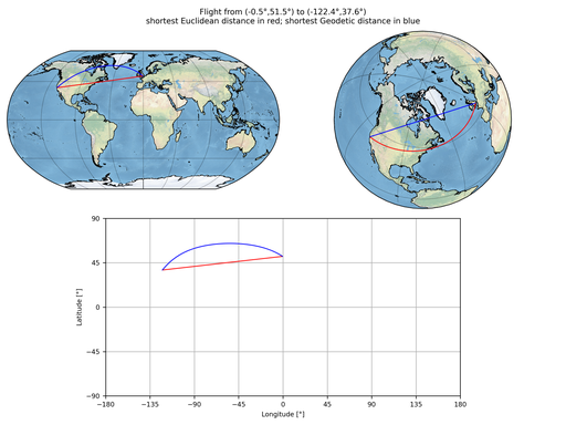
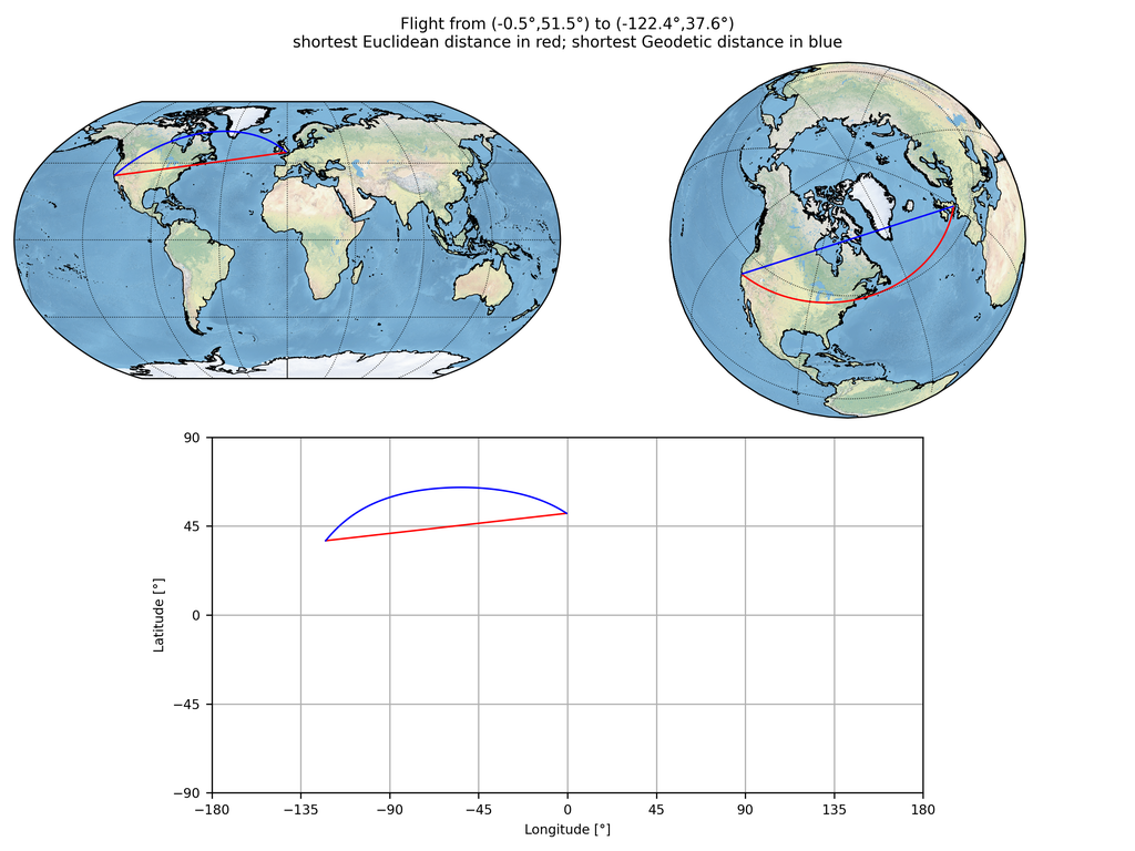
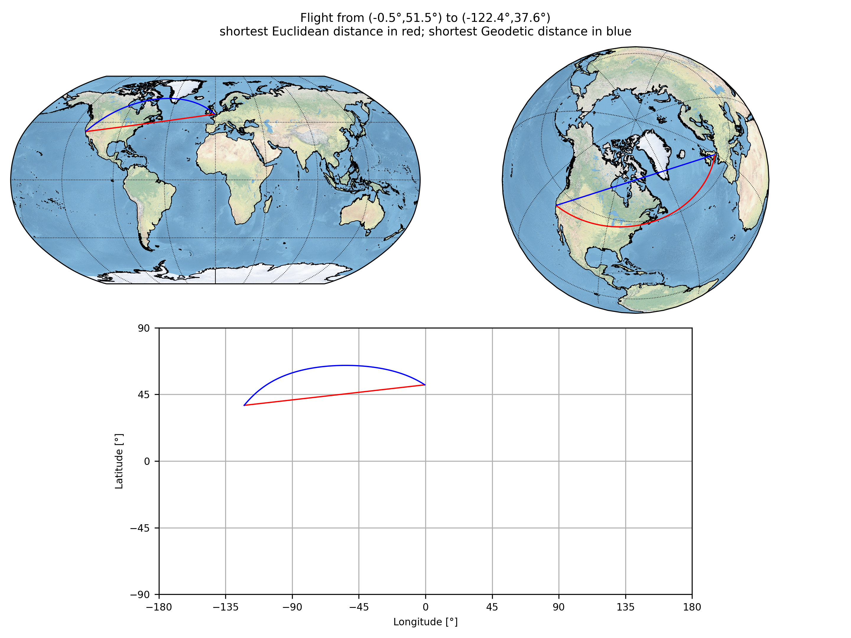
This difference is best highlighted by aeroplanes: aeroplanes fly in a straight line from point A to point B over the surface of the Earth. Depending on the map projection that is used, this line appears curved. These lines are called great circles. For example, consider the flight from London to San Francisco:

Here is the Python script to create the above map:
1 2 3 4 5 6 7 8 9 10 11 12 13 14 15 16 17 18 19 20 21 22 23 24 25 26 27 28 29 30 31 32 33 34 35 36 37 38 39 40 41 42 43 44 45 46 47 48 49 50 51 52 53 54 55 56 57 58 59 60 61 62 63 64 65 66 67 68 69 70 71 72 73 74 75 76 77 78 79 80 81 82 83 84 85 86 87 88 89 90 91 92 93 94 95 96 97 98 99 100 101 102 103 104 105 106 107 108 109 110 111 112 113 114 115 116 117 118 119 120 121 122 123 124 125 126 127 128 129 130 131 132 133 134 135 136 137 138 139 140 141 142 143 144 145 146 147 148 149 150 151 152 153 154 155 156 157 158 159 160 161 162 163 164 165 166 167 168 169 170 171 172 173 174 175 176 177 178 179 180 181 182 183 184 185 186 187 188 189 190 191 192 193 194 195 196 197 198 199 200 201 202 203 204 205 206 207 208 209 210 211 212 213 214 215 216 217 218 219 220 221 222 |
|
checkout the “main” branch).In the above map, the red line is the line connecting (-0.4619°,51.4706°) and (-122.3750°,37.6180°) in Euclidean space, i.e., treating all degrees as being of equal size in all directions. The blue line is the line connecting (-0.4619°,51.4706°) and (-122.3750°,37.6180°) in Geodesic space, i.e., having knowledge that the degrees actually describe a location on the surface of a spheroid and that degrees have different physical size depending on where you are and which direction you are pointing. The above script also reports that:
- The shortest line in Euclidean space (in red) is 122.7° long and 9,786,917.7m long.
- The shortest line in Geodesic space (in blue) is 132.1° long and 8,638,329.4m long.
This demonstrates why aeroplanes fly the large arcs that they do: the red line is 1,148,588.3 metres shorter than the blue line, but it is also 9.4° longer. As a passenger on an aeroplane, which one of those two differences is more important to you?
§4 Tissot’s Indicatrix
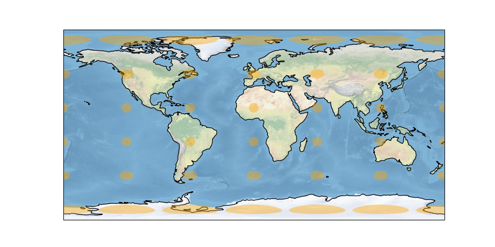
In the above map, the red and blue lines appear differently depending on the map projection that is used. No map projection is perfect, just see xkcd for some hilarious examples. As a way of displaying how distorted, or not, a map projection is Tissot’s indicatrix are sometimes displayed on a map. These are simply circles which have a constant radius in metres and which, therefore, appear distorted on the surface of the Earth. Cartopy has an example script which displays Tissot’s indicatrix and produces the below map.

Here is the Python script to create the above map:
1 2 3 4 5 6 7 8 9 10 11 12 13 14 15 16 17 18 19 20 21 22 23 24 25 26 27 28 29 30 31 32 |
|
checkout the “main” branch).§5 Vincenty’s Formulae
… and now all the way back to me mentioning Vincenty’s formulae in the introduction. Vincenty’s formulae are iterating functions which perform two tasks:
- given two points defined using longitude and latitude in degrees: find the bearing from the first to the second in degrees; find the bearing from the second to the first in degrees; and find the distance between the two in metres (a.k.a “the inverse problem”)
- given a starting point defined using longitude and latitude in degrees and a bearing in degrees and a distance in metres: find the end point’s longitude and latitude in degrees and the bearing back to the start in degrees (a.k.a “the direct problem”)
If you wanted to create your own Tissot’s indicatrix manually then all you would need to do is pick a starting location and call “the direct problem” of Vincenty’s formulae for a list of bearings (with a constant distance) to obtain a list of end locations. These end locations are the circumference of a circle used in Tissot’s indicatrix. You can then repeat the process for different starting locations to populate the whole map projection.
If you look at the source code of the tissot() method you will see that it calls the circle() method in the Geodesic class. If you look at the source code of the Geodesic class then you will see that Cartopy just calls its own implementation of “the direct problem”.
§6 Buffering
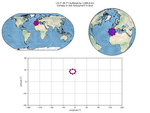
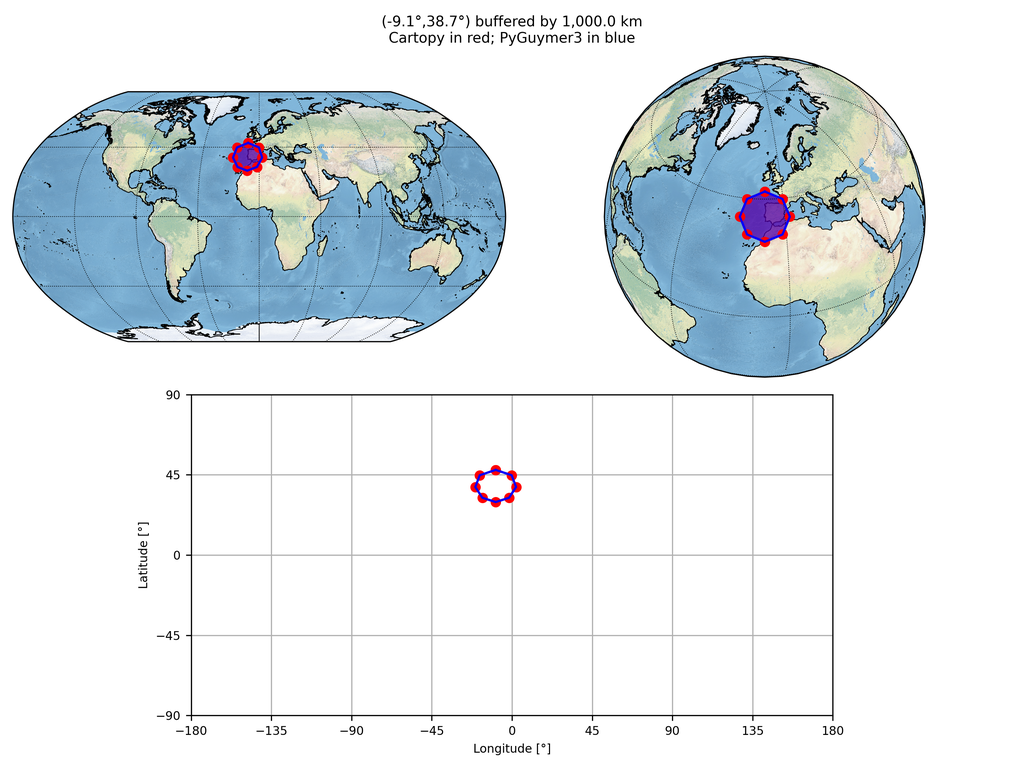
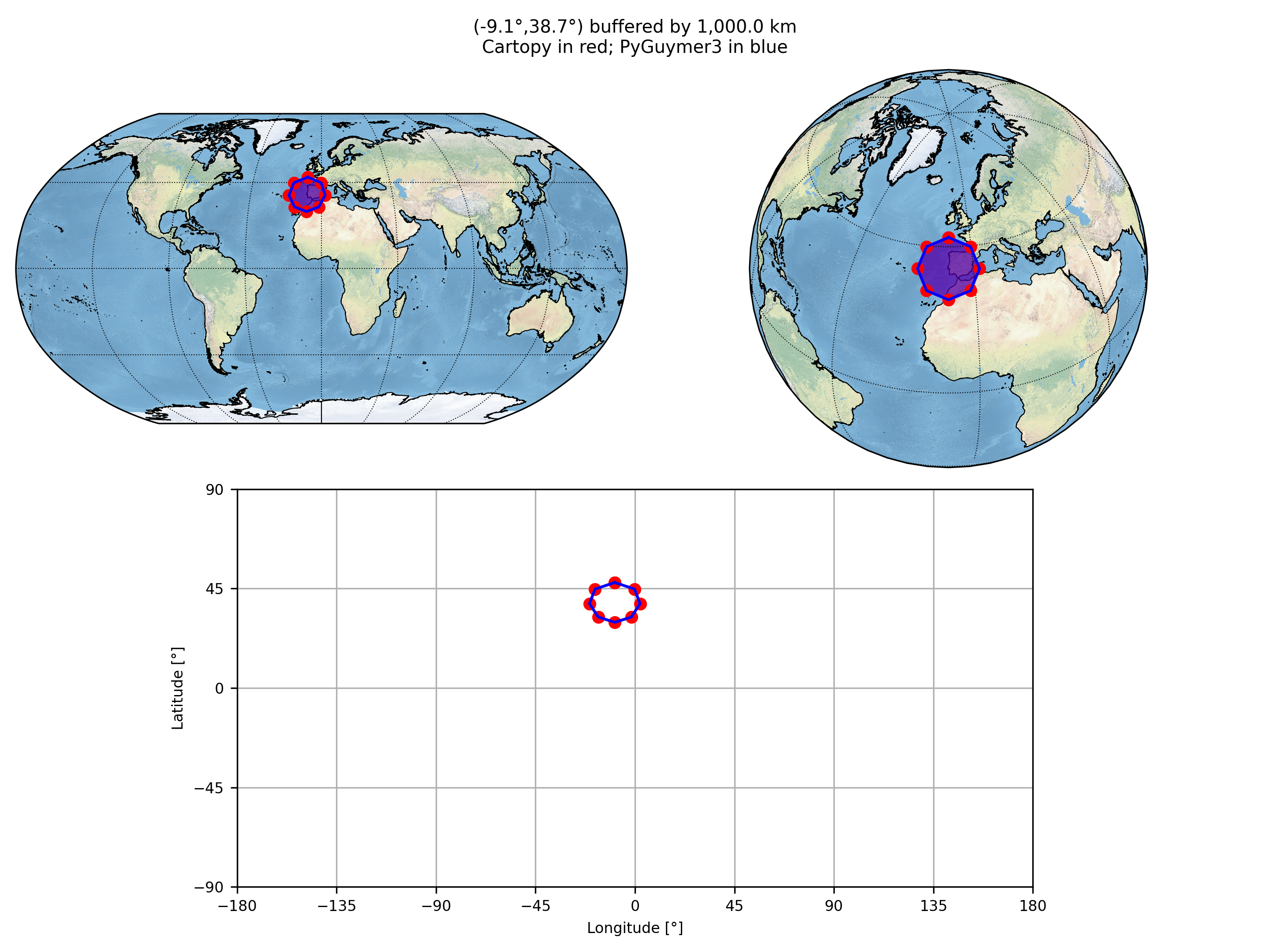
The below map shows Lisbon buffered by 1,000.0 kilometres by both Cartopy and my Python 3 module. Reassuringly, they both give the same answer.

Here is the Python script to create the above map:
1 2 3 4 5 6 7 8 9 10 11 12 13 14 15 16 17 18 19 20 21 22 23 24 25 26 27 28 29 30 31 32 33 34 35 36 37 38 39 40 41 42 43 44 45 46 47 48 49 50 51 52 53 54 55 56 57 58 59 60 61 62 63 64 65 66 67 68 69 70 71 72 73 74 75 76 77 78 79 80 81 82 83 84 85 86 87 88 89 90 91 92 93 94 95 96 97 98 99 100 101 102 103 104 105 106 107 108 109 110 111 112 113 114 115 116 117 118 119 120 121 122 123 124 125 126 127 128 129 130 131 132 133 134 135 136 137 138 139 140 141 142 143 144 145 146 147 148 149 150 151 152 153 154 155 156 157 158 159 160 161 162 163 164 165 166 167 168 169 170 171 172 173 174 175 176 177 178 179 180 181 182 183 184 185 186 187 188 189 190 191 192 193 194 195 196 197 198 199 200 201 202 203 204 205 206 207 208 209 210 211 212 213 214 215 216 217 218 219 220 221 222 223 |
|
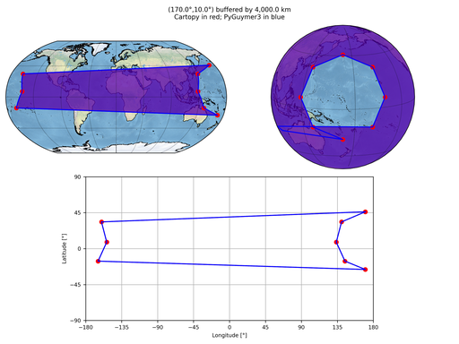
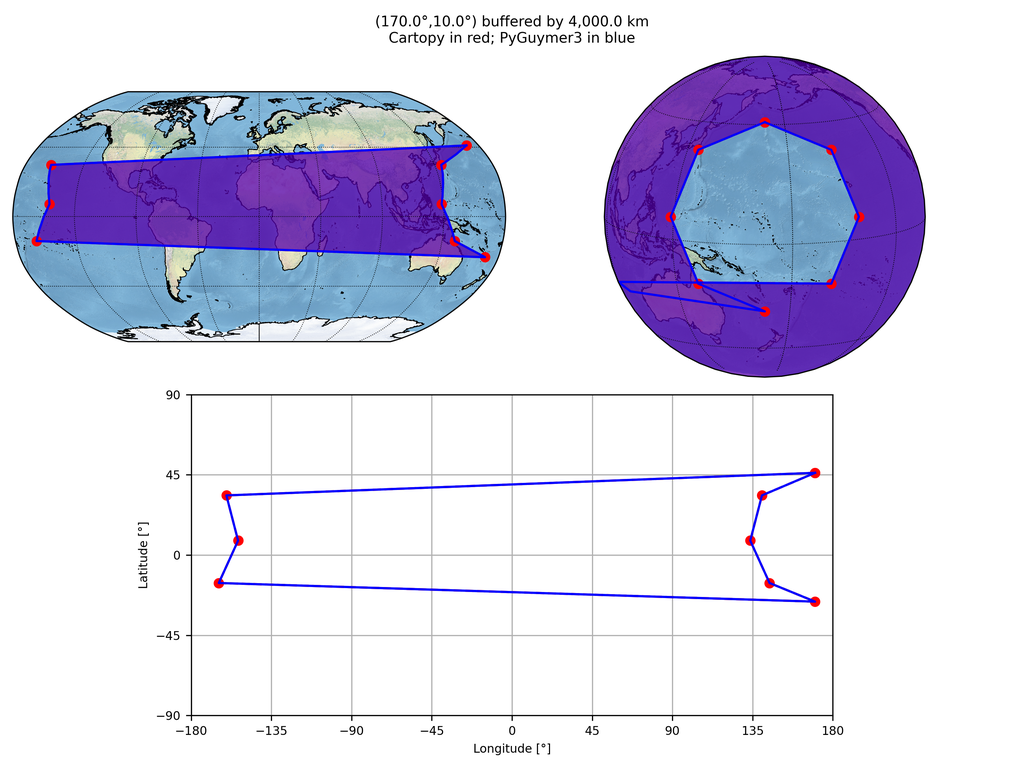
checkout the “main” branch).Now, if I try the same script but using a random point in the middle of the Pacific Ocean then things go horribly wrong.

Here is the Python script to create the above map:
1 2 3 4 5 6 7 8 9 10 11 12 13 14 15 16 17 18 19 20 21 22 23 24 25 26 27 28 29 30 31 32 33 34 35 36 37 38 39 40 41 42 43 44 45 46 47 48 49 50 51 52 53 54 55 56 57 58 59 60 61 62 63 64 65 66 67 68 69 70 71 72 73 74 75 76 77 78 79 80 81 82 83 84 85 86 87 88 89 90 91 92 93 94 95 96 97 98 99 100 101 102 103 104 105 106 107 108 109 110 111 112 113 114 115 116 117 118 119 120 121 122 123 124 125 126 127 128 129 130 131 132 133 134 135 136 137 138 139 140 141 142 143 144 145 146 147 148 149 150 151 152 153 154 155 156 157 158 159 160 161 162 163 164 165 166 167 168 169 170 171 172 173 174 175 176 177 178 179 180 181 182 183 184 185 186 187 188 189 190 191 192 193 194 195 196 197 198 199 200 201 202 203 204 205 206 207 208 209 210 211 212 213 214 215 216 217 218 219 220 221 222 223 |
|
checkout the “main” branch).Shapely tries to make a polygon from the list of points along the ring, but it has no idea about the anti-meridian and so whilst it does make a mathematically correct polygon it is certainly not the one that the user desired. In summary, Vincenty’s formulae correctly return the longitudes and latitudes of all of the points along a ring which is a fixed distance (in metres) around a point but assembling these points into a polygon in Shapely is not trivial when the ring crosses either the anti-meridian or one of the poles.
Therefore, a function needs writing which takes the raw list of longitude and latitude pairs and uses them to create a polygon for the user. This function needs to be clever enough to return two individual polygons when the ring around a point crosses either the anti-meridian or one of the poles. I wrote a function to perform this task and it served me well for numerous years, such as:
- performing complex buffering when finding antipodes in How To Avoid Places
- performing complex buffering when finding ranges from airfields in What Are The Ranges From British Airfields?
- performing simple buffering when drawing attention a location in Using Ordnance Survey Images As Backgrounds In Cartopy
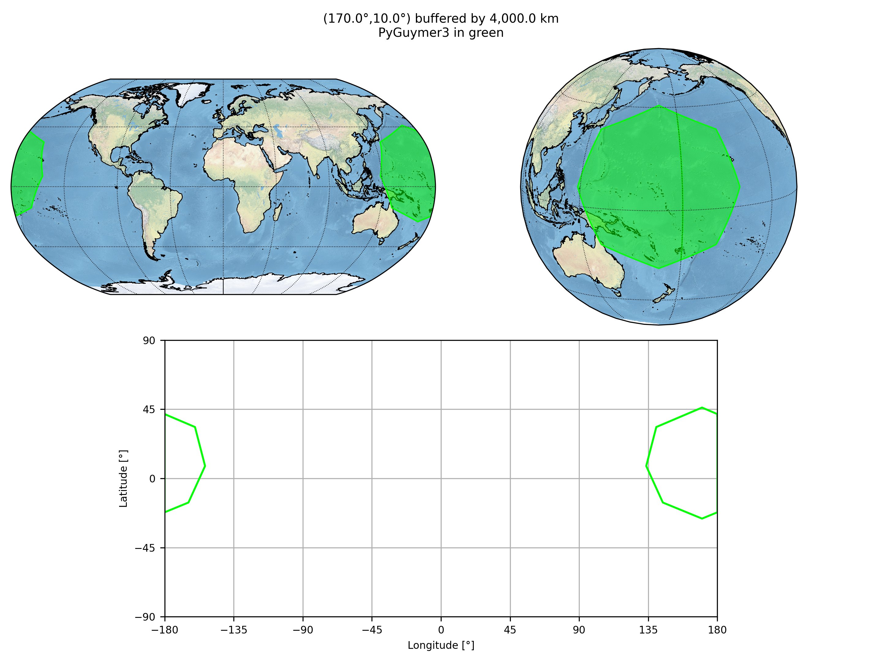
However, it was not completely robust and as I worked on ever more complex projects I found sets of input values which would break it. I believe that my new function pyguymer3.geo._points2polys() works more robustly than any of the other ones that I have written over the years. For example, see how it fixes the buffered point in the Pacific Ocean (from above) by returning two unconnected polygons:

Here is the Python script to create the above map:
1 2 3 4 5 6 7 8 9 10 11 12 13 14 15 16 17 18 19 20 21 22 23 24 25 26 27 28 29 30 31 32 33 34 35 36 37 38 39 40 41 42 43 44 45 46 47 48 49 50 51 52 53 54 55 56 57 58 59 60 61 62 63 64 65 66 67 68 69 70 71 72 73 74 75 76 77 78 79 80 81 82 83 84 85 86 87 88 89 90 91 92 93 94 95 96 97 98 99 100 101 102 103 104 105 106 107 108 109 110 111 112 113 114 115 116 117 118 119 120 121 122 123 124 125 126 127 128 129 130 131 132 133 134 135 136 137 138 139 140 141 142 143 144 145 146 147 148 149 150 151 152 153 154 155 156 157 158 159 160 161 162 |
|
checkout the “main” branch).§7 Testing
my Python 3 module contains a couple of test scripts (“bufferPoint” and “buffer”) which have slowly ballooned to contain new inputs which demonstrate previous shortcomings and which hope to guard against future regressions in robustness. After growing tired of adding yet more examples to these scripts, I decided to write a third script which just loops over all combinations of longitude and latitude on Earth in an effort to pre-emptively catch further errors: “animateBufferPoint”. I am pleased to include the video below, which has been generated by this testing script of my new function:
As you can see, across all locations on the surface of the Earth, the function is able to take the longitude and latitude pairs and correctly generate one or two Shapely polygons which correctly describe what the user is expecting: a perfect circle around a point with a fixed radius, defined in metres. Whether this point is near to one of the Poles or near to the anti-meridian is irrelevant: when viewed from an orthographic projection above the point then the circle appears as a circle. There are no glitches or weird bumps or excursions in the polygon(s).
Buffering a polygon is similarly straightforward: just split the polygon up into its individual points (on its exterior and its interiors) then return the union of these buffers with the original polygon.
§8 Summary
In summary, after over five years of writing “geospatial themed” Python scripts, I believe that I now have a robust Python function which can return one or two Shapely polygons of the buffer around a point on the surface of the Earth. With the tests scripts that are part of my my Python 3 module module, I believe that this function (and its wrappers) works correctly for all locations on the surface of the Earth.