My Blog

On the 23^rd of March 2021 a container ship ran aground in the Suez Canal. It was freed on the 29^th of March 2021 and it was eventually released by the Egyptian government on the 7^th of July 2021, after which, it proceeded on its journey. The whole saga caused massive disruption to global shipping as it forced container ships to divert around Africa instead of sailing through the Suez Canal. At the time, various numbers were floated about how much longer it takes to sail around Africa rather than through the Suez Canal. These numbers always seemed over-simplified to me as they never caveated themselves enough about the exact source and destination of shipping routes: the exact benefit of the Suez Canal depends on where you are going and where you have come from.

I decided to create some software to calculate the sailing times from any point in the world: GST (Global Sailing Times). This blog post describes how it works, some of the pitfalls of calculating something so complicated so generically and then reports some results of sailing around the world from Portsmouth. This project has only been made possible by my recent blog post on reliably buffering a shape (in fact, it was creating this project which forced me to improve my functions so that they are reliable).

§1 Basic Method

The method employed by GST is conceptually very simple:

1. define the ship’s starting Point;
2. buffer the ship’s starting Point by a Geodetic distance (thus creating a Polygon);
3. subtract any land which overlaps with the ship’s Polygon; then
4. keep on buffering/subtracting the ship’s Polygon until it has grown to cover all sailable sea(s).

The only extra step required is that the Polygons which describe the land cannot have any narrow headlands/spits which are narrower than the buffering distance, otherwise the ship will jump over them rather than sailing around them. Therefore, the land itself needs buffering initially too. In effect, this is simply saying that the ship cannot sail too close to shorelines.

You can imagine that whilst this method is very simple, providing that you can reliably buffer a Point/Polygon, it could have lots of choices involved about how large the steps are, how detailed the land is, etc … which can strongly affect calculation time.

§2 Shoreline Dataset

For this project I chose to use the GSHHG (Global Self-Consistent Hierarchical High-Resolution Geography) shorelines dataset, which instantly opened up a choice to the user: what resolution should be used? Within the GSHHG shorelines dataset there are five resolutions to choose from:

• crude (“c”);
• low (“l”);
• intermediate (“i”);
• high (“h”); and
• full (“f”).

The animation below shows what the shorelines around Portsmouth look like for these five different resolutions. The “c” resolution is really quite crude - the Isle Of Wight is little more than a line!

Within the GSHHG shorelines dataset there are six levels to choose from too:

• boundary between land and ocean (1);
• boundary between lake and land (2);
• boundary between island-in-lake and lake (3);
• boundary between pond-in-island and island-in-lake (4);
• boundary between Antarctica ice and ocean (5); and
• boundary between Antarctica grounding-line and ocean (6).

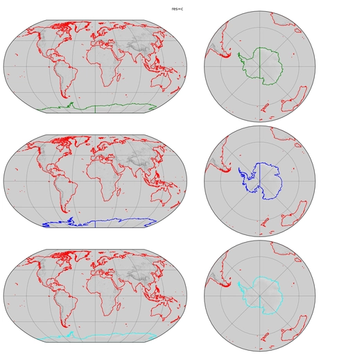
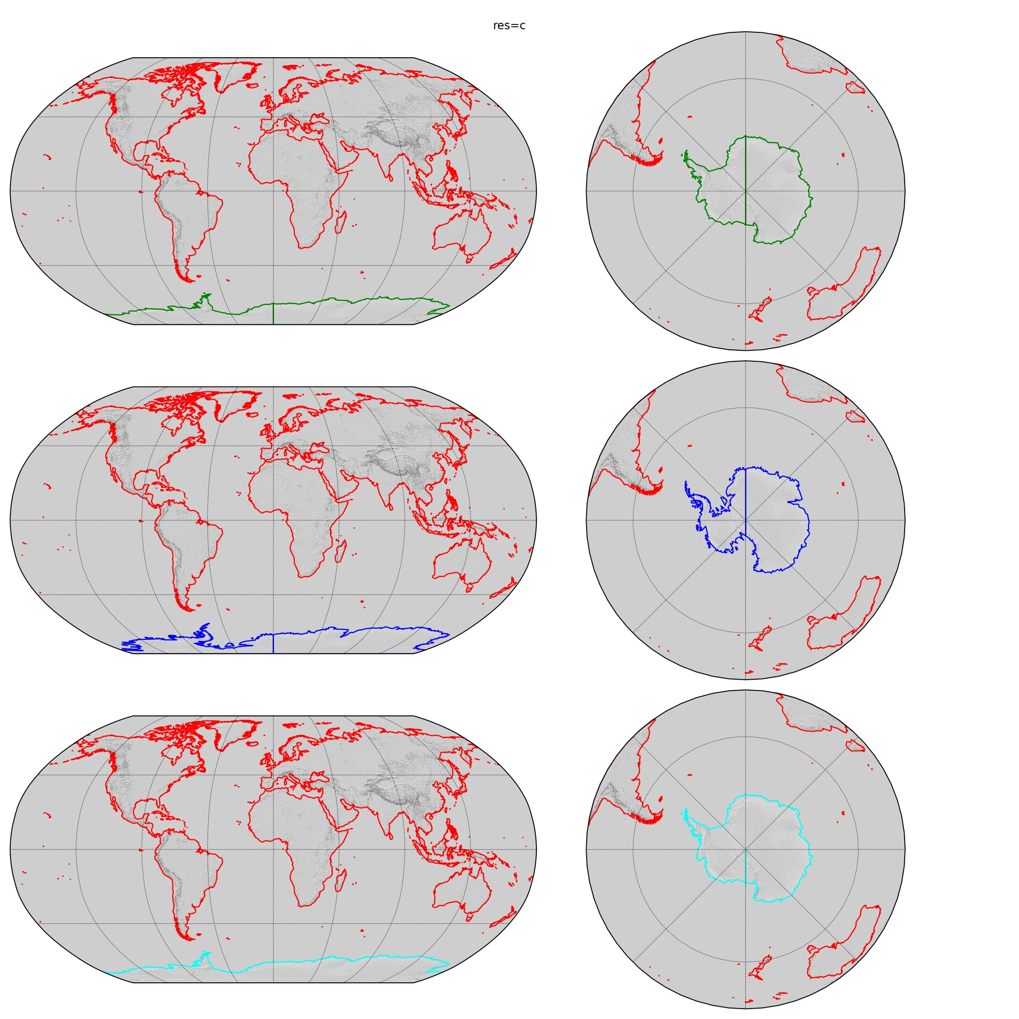
Upon first consideration, you may think that the boundaries that are needed are between land and ocean (1) and between Antarctica ice and ocean (5). However, at the full resolution there is a bug in the shoreline of Antarctica which cannot be easily fixed. Therefore, I also include the boundary between Antarctica grounding-line and ocean (6) and merge all three levels together (rather than just merging level 1 and level 5 together). This is demonstrated in the animation below: red boundaries are level 1; green boundaries are level 5; blue boundaries are level 6; and cyan boundaries are the union of levels 5 and 6. Note how a huge chunk of land is cut out of Antarctica in the green boundary when displaying the full resolution in the upper-right subplot.

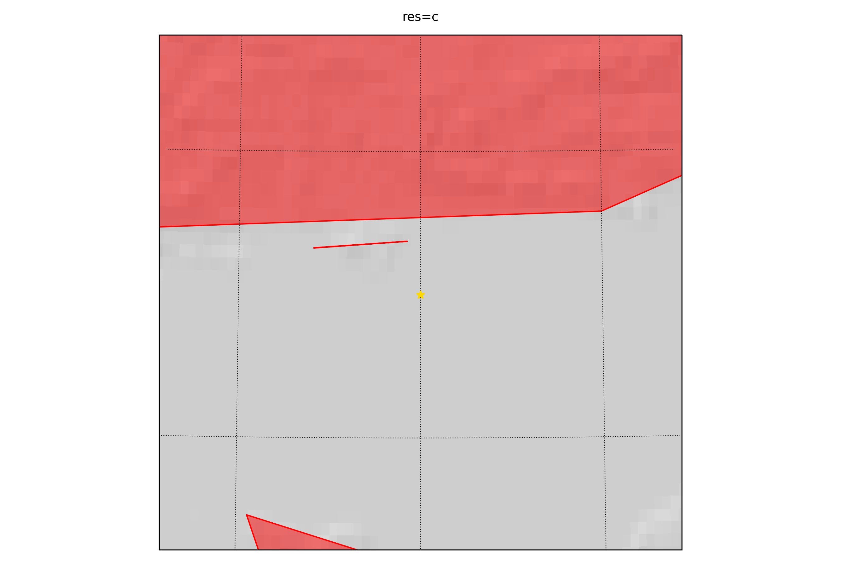
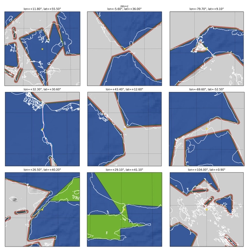
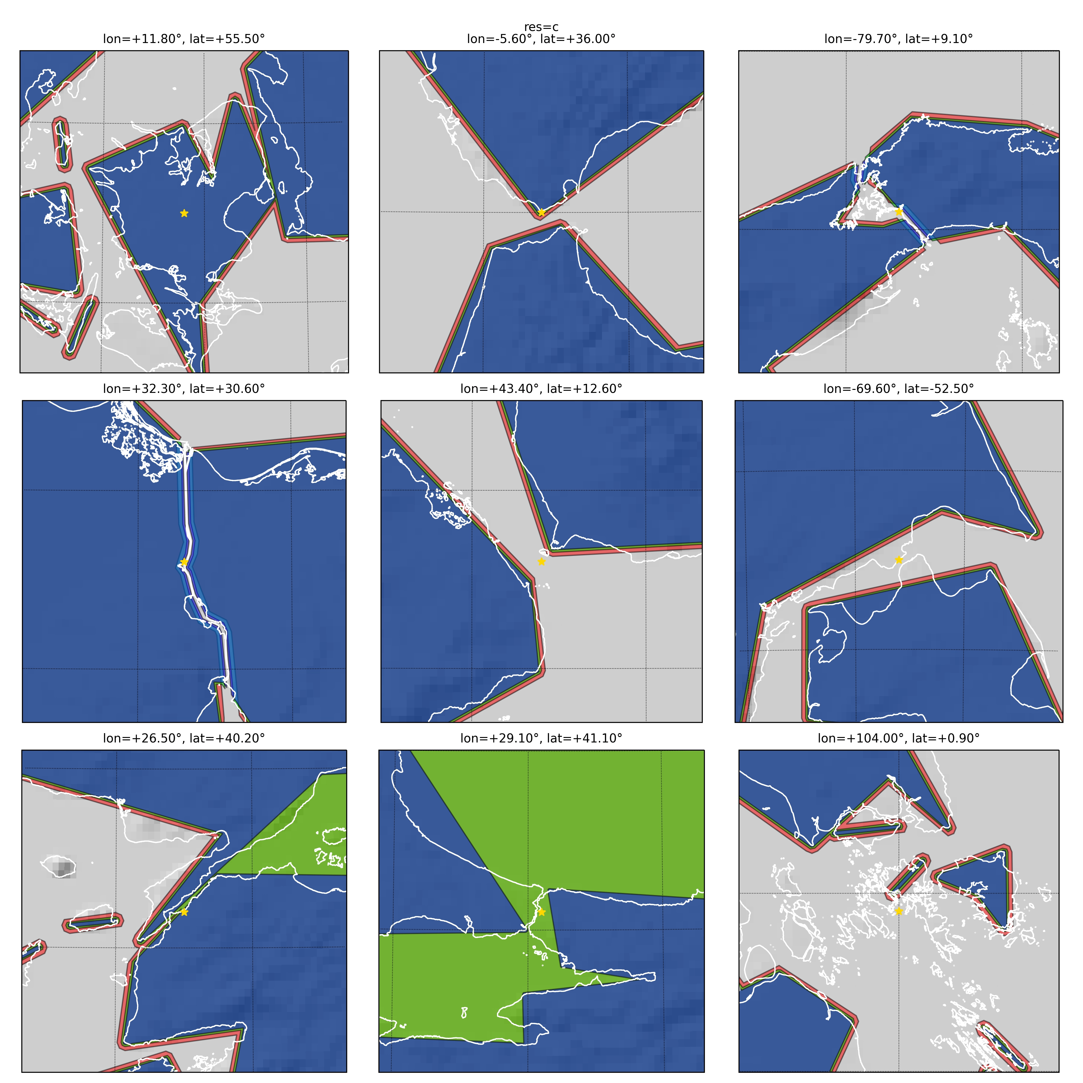
Finally, the aforementioned trick of buffering the land to avoid the ship jumping over narrow spits of land has the detrimental effect of closing off some narrow passages. The below animation shows a selection of narrow passages around the world for a variety of GSHHG shorelines dataset resolutions and pyguymer3.geo.buffer() settings. The “Rivers and Lake Centerlines” Natural Earth dataset is used to ensure that the Panama Canal and Suez Canal are always kept open; other passages (such as The Dardanelles in the lower-left subplot) are at the mercy of the user.

Some narrow passages are closed off by the buffering, particularly at higher resolutions when more tiny islands are included in the GSHHG shorelines dataset. Some of these will affect the routes that the ship can sail around the world - others just make certain ports inaccessible (such as Istanbul in the lower-centre subplot).

After all of the processing to obtain a useable dataset of the coastlines, an important consideration is how many points are used to describe the coastlines. Some places in the world will have more points to describe their coastlines than others. This can significantly affect run time later on. For different levels of processing quality, here are maps of the number of points in the coastline dataset around the world.

At the highest fidelity settings, the region near the Western coast of North Korea has the highest concentration of points, which was unexpected.

§3 Angular Convergence

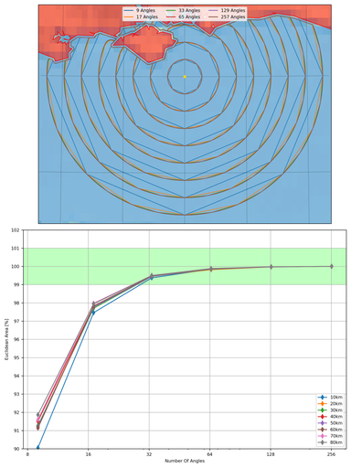
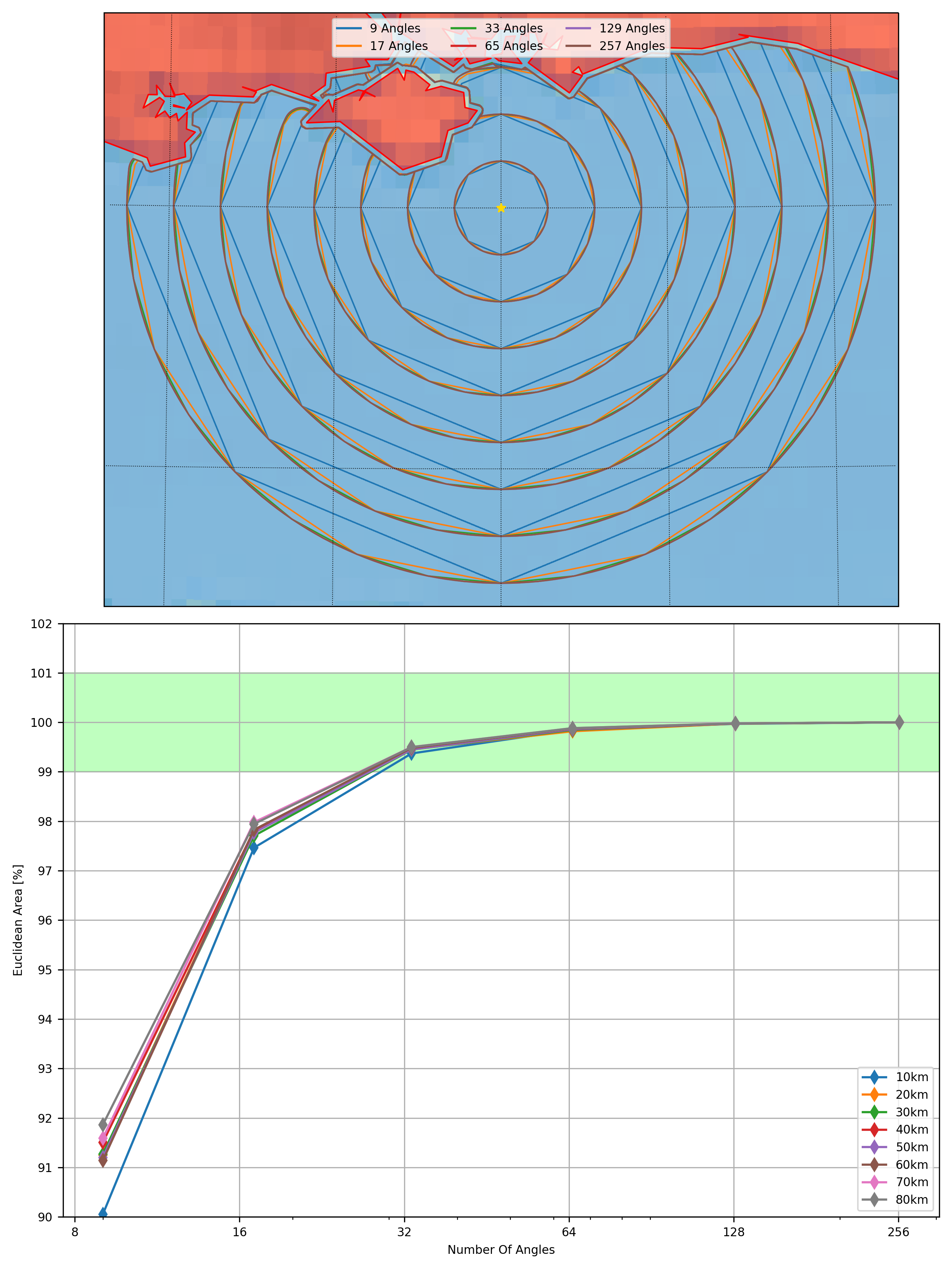
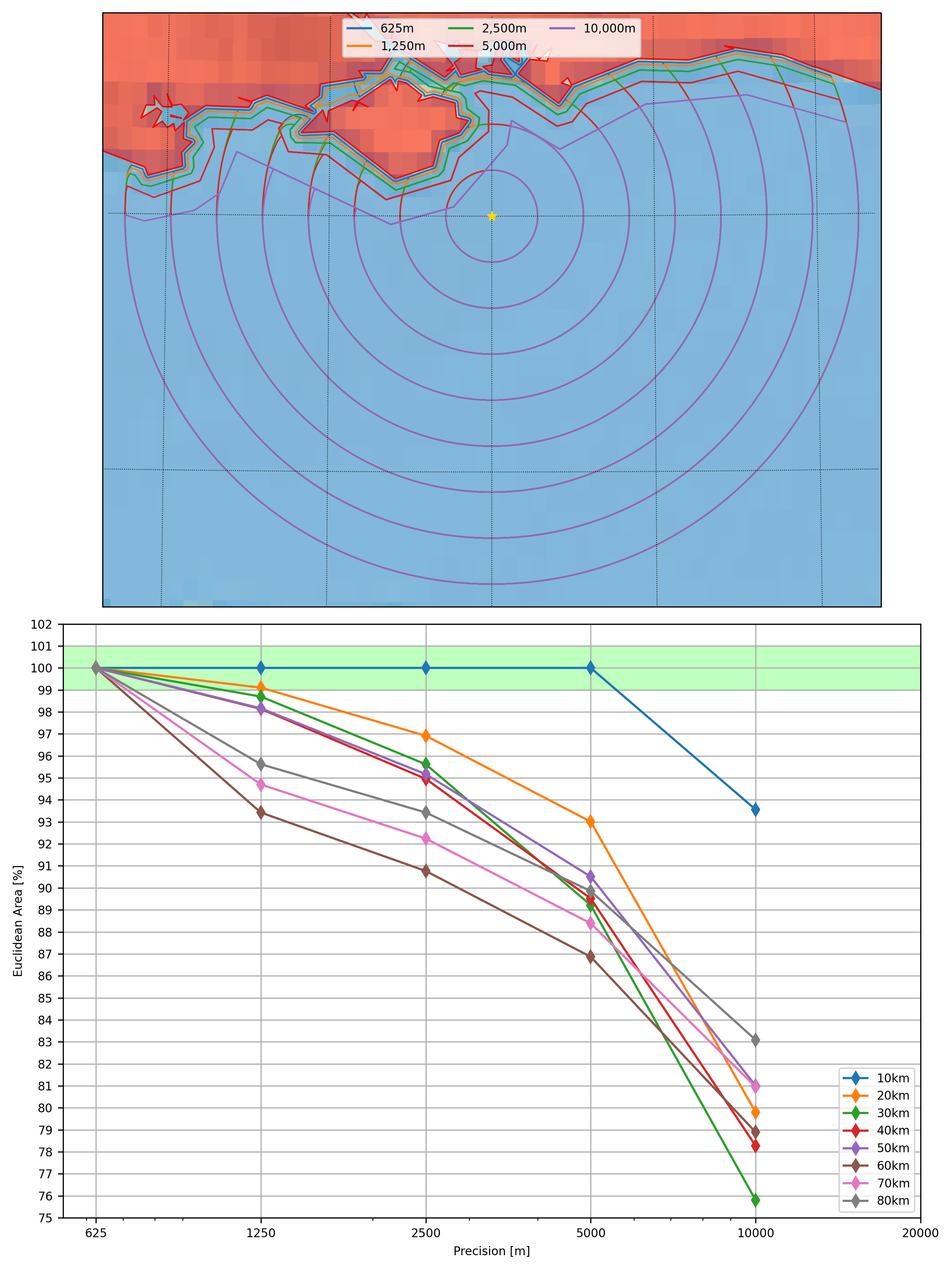
When pyguymer3.geo.buffer() is called, there is an argument called nang, which is the number of angles around a point to populate when buffering a point. The higher the number the smoother the exterior of the Polygon is, however, computational time and memory usage will go up. Furthermore, owing to the loop in the basic method outlined above, the value of nang determines how many starting points there are on the next iteration, so nang exponentially affects computational time and memory usage when sailing a ship. The map below shows how nang affects ships sailing out of Portsmouth.

Unsurprisingly, the biggest difference between the different values of nang is how well the ship sails around corners. This is particularly obvious at the very Western tip of The Isle Of Wight. The user must make a trade between run time and quality of the final answer.

The lower plot shows how the Euclidean area of the Polygons converges as a function of nang. A value of 33 is within 1% of the “correct” answer, and will be used as the “best” value later on.

§4 Radial Convergence

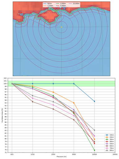
When performing the loop in the basic method outlined above, the user can choose the step size, i.e., how far to sail the ship in a single iteration before calculating the next iteration. The smaller the distance the smaller the buffering of the land (and hence the less likely it is that narrow passages will be closed off), however, computational time will go up. Furthermore, owing to the loop in the basic method outlined above, the step size linearly affects computational time when sailing a ship. The map below shows how the step size affects ships sailing out of Portsmouth.

Unsurprisingly, the biggest difference between the different step sizes is how well the ship sails between land. This is particularly obvious along the Northern coast of The Isle Of Wight. The user must make a trade between run time and quality of the final answer.

The lower plot shows how the Euclidean area of the Polygons converges as a function of step size. This plot is more nuanced than the earlier one: here, comparing each Polygon is unfair as they are each seeing differently buffered land. (Additionally, buffering by 625 metres is not enough to join The Isle Of Wight to the mainland, therefore, the lines for “60km”, “70km” and “80km” have a different convergence/shape to the others as GST has deleted the interior void of The Isle Of Wight once it became completely encompassed by the ship.) When picking a step size it is perhaps better to make your decision on how it affects the narrow passages that you are interested in rather than the Euclidean area of the Polygons. A value of 1.25 kilometres will be used as the “best” value later on.

§5 Conservatism

GST also has a conservatism argument, which is a fudge factor for how much more resolution should be applied to ensure that the final answer looks good. This section will use the example of sailing out from Portsmouth at 20 knots for 6 days and seeing where the ship ends up.

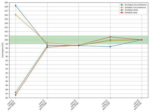
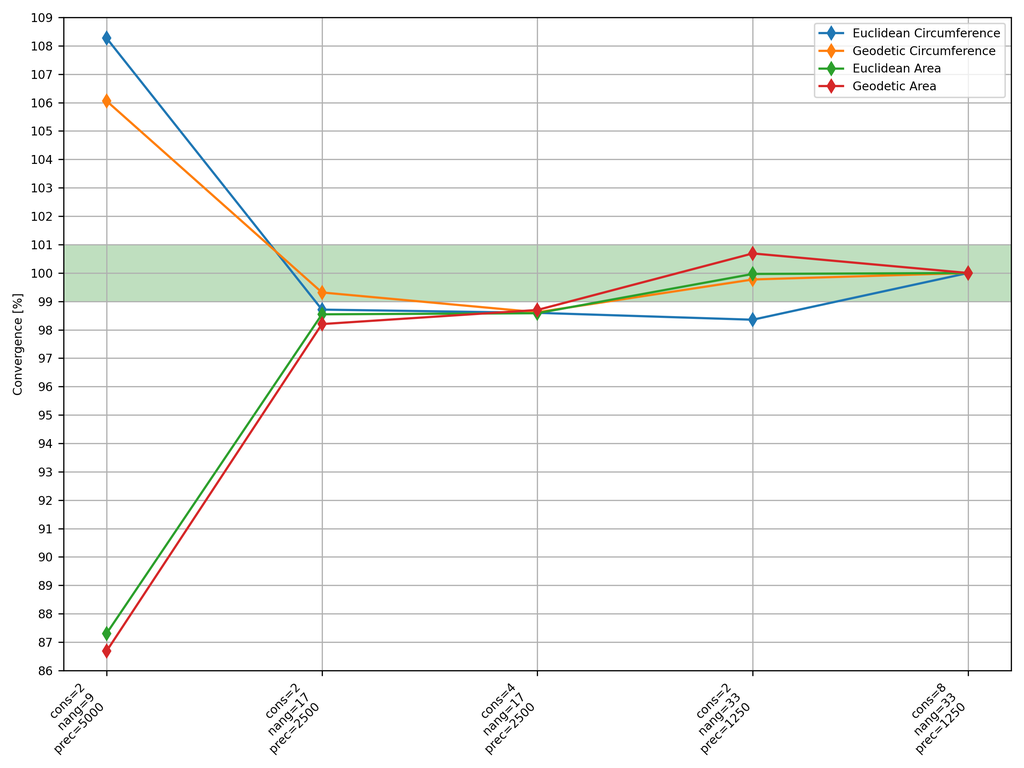
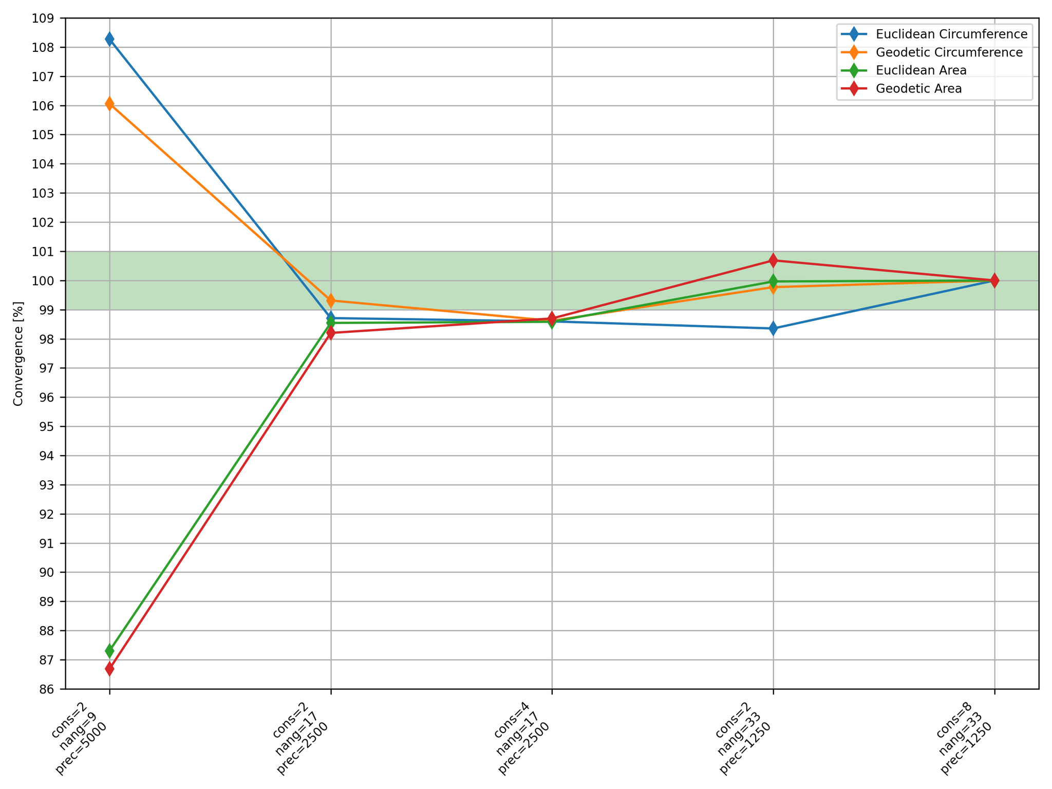
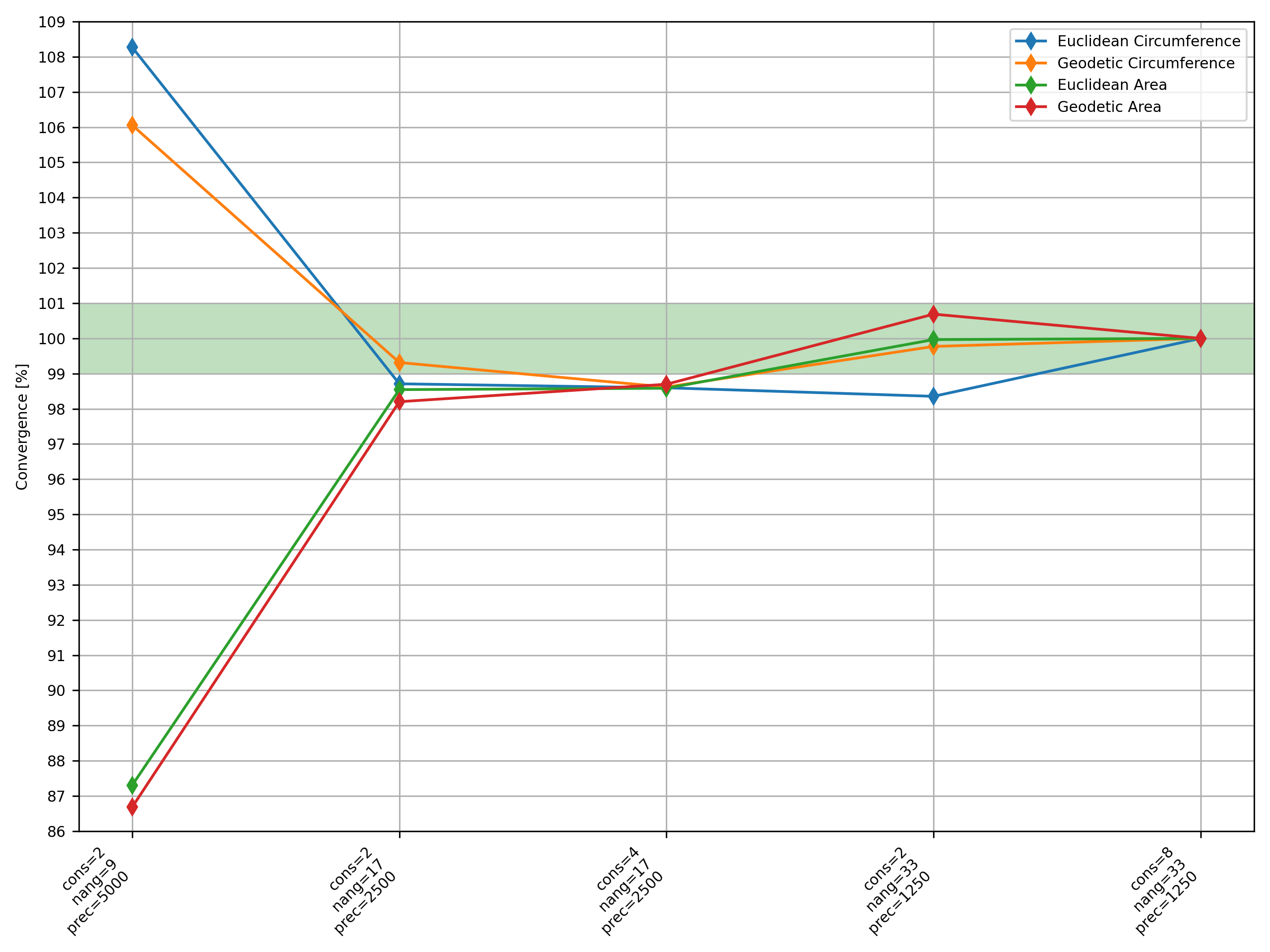
The below plot compares four different metrics of the final Polygon for a series of different runs of GST. Here: nang is the number of angles (as described above); prec is the step size (as described above) in metres; and cons is the conservatism (a value of 1.0 is no conservatism). After the plot, there are a series of videos comparing the different runs of GST further.

The below video compares:

• cons=2.0; nang=9; prec=5000.0
• cons=2.0; nang=17; prec=2500.0
• cons=2.0; nang=33; prec=1250.0

The below video compares:

• cons=2.0; nang=9; prec=5000.0
• cons=4.0; nang=17; prec=2500.0
• cons=8.0; nang=33; prec=1250.0

The below video compares:

• cons=2.0; nang=17; prec=2500.0
• cons=4.0; nang=17; prec=2500.0

The below video compares:

• cons=2.0; nang=33; prec=1250.0
• cons=8.0; nang=33; prec=1250.0

Watching the last two videos shows that at decent values of nang and prec there is no visual benefit to having more conservatism than simply a factor of two. Using the first plot, and taking the “cons=8.0; nang=33; prec=1250.0” combination as “correct”, then for the four metrics:

• “cons=2.0; nang=9; prec=5000.0” is converged to between 6% and 13%;
• “cons=2.0; nang=17; prec=2500.0” is converged to between 1% and 3%; and
• “cons=2.0; nang=33; prec=1250.0” is converged to between 0% and 2%.

These are the three combinations that I will be using for my final results later on.

§6 Internal Voids

The Matochkin Strait, within the Novaya Zemlya archipelago, is yet another example of a narrow passage which gets closed off by the initial buffering of the land: it is approximately 600 metres wide at its narrowest point. Additionally, it is frozen over for most of the year; GST is not aware of frozen seas (it treats all seas as perfectly navigable). However, it is most interesting here because it shows an early example of how sailing around land can create holes in the ship’s Polygon. This demonstrates why, when writing GST, I could not save computational time by only buffering the exterior of the ship’s Polygon - I must also buffer each interior ring until it explicitly closes off.

Note how when the ship sails round the Southern and Northern tips of Novaya Zemlya, and then sails North and South on the open sea to meet itself, it creates a void to the West (on the East coast of Novaya Zemlya) which it must take some time to sail into. This would not have been captured if I had deleted all internal voids.

Also note how the above video excellently demonstrates that low values of nang and high values of prec result in a ship which sails around land very poorly: the red Polygon lags behind the green and blue Polygons by an awfully long way.

Another excellent example is the Boca Del Guafo. The area of sea south of the main port of Puerto Montt has a really quite complicated coastline and also is very close to where a ship sailing south from the Panama Canal collides with a ship sailing north from the Magellan Straits.

§7 Results

After all the above waffle, here are the final results:

The above video clearly demonstrates the benefit of both the Panama Canal and the Suez Canal. I am particularly impressed by the Panama Canal: from Portsmouth it basically doesn’t have any delay. Conversely, the Suez Canal does still have quite a delay, but this is due to France and Spain getting in the way and the ship having to sail the whole length of the Mediterranean. Interestingly, by the time the ship gets very close to the end, it hasn’t used any canal to get there: it has simultaneously gone over the North Pole and gone around the Horn Of Africa and Cape Horn. It really does depend on where you are going as to how useful the two canals are. Finally, the above video really does show the potential benefits to global shipping if the Northwest Passage opens up (frankly though, I would prefer it to stay closed: having a non-warming planet is better than slightly quicker global sailings).

As an aside, The CIA World Factbook has a nice PDF map of the world oceans and shipping routes which aligns nicely with the conclusions in this article.

§8 Diagnostics

I am embarrassed to say that GST took quite a long time to calculate the “best” combination in the above video (ironically, it isn’t the buffering that takes ages, it is the subtracting of land from the ship). Whilst it was running, I wrote some scripts to diagnose the complexity of the problem.

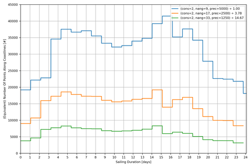
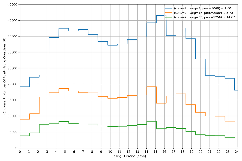
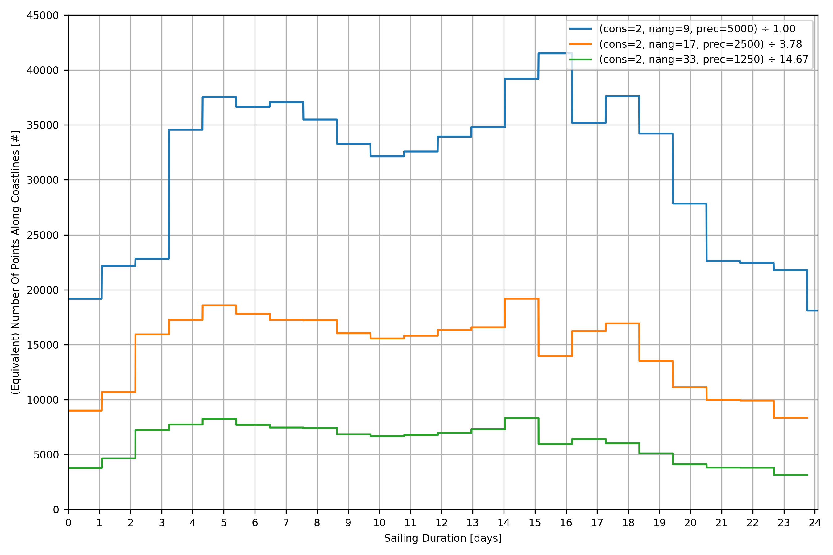
Firstly, how many Points are there along the coastlines?

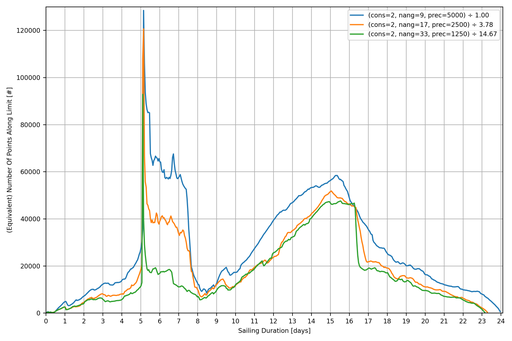
Secondly, how many Points are there around the ship?

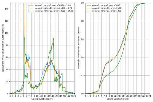
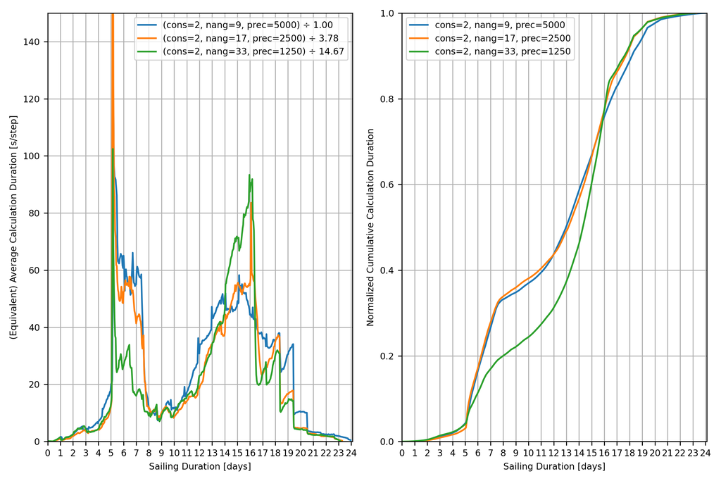
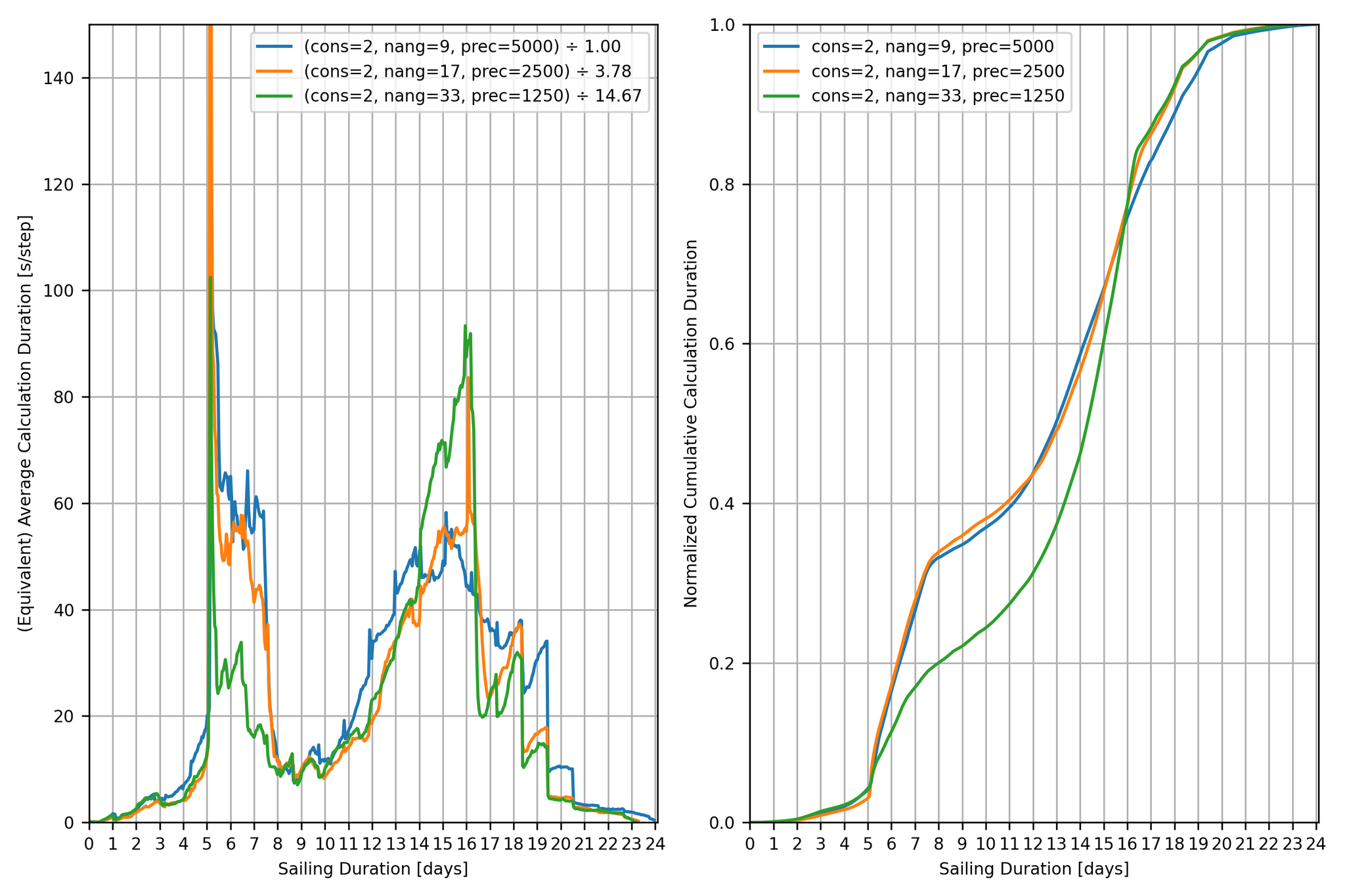
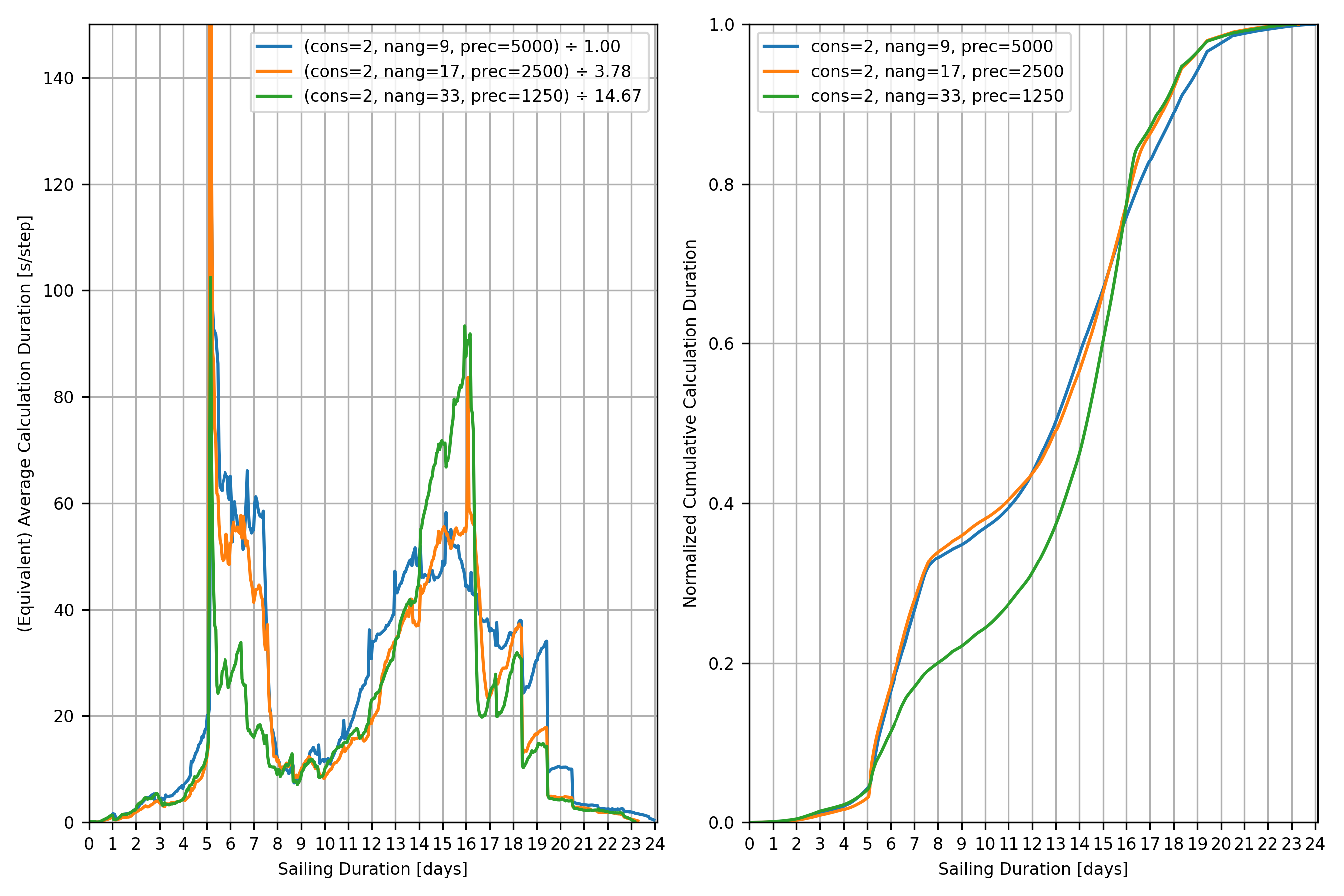
Thirdly, how long does it take to calculate each iteration step?

The spike at 5 days is the point where the ship crosses the North Pole (and the mapping between degrees and metres becomes degenerate). The drop at 16 days is the point where South America gets deleted as it has been completely encompassed by the ship.